Crosssum Analytics
Cross-summing numbers tell us a lot about the qualitative nature of numbers, rather that the quantitative.
Cross-summing two unrelated numbers like a carnival numerologist will generate seemingly meaningless data, at least with respect to the quantitative significance of that data, but it will have plenty of information about how each number relates to the others, regardless of the source of the data. Even with perfectly random numbers, as a cross-sum that is divisible by 3 means the entire number is divisible by 3, and if divisible by 9 then than entire number is divisible by 9. We all know that if the last digit of a number is 2, then that number is divisible by 2, but it is also true if the cross-sum of the last 2 digits of a number equals 4, then that number is divisible by 4. Testing for divisible by 8 can also be done by cross-sums, but is a bit more complicated. You join the 2 leftmost numbers and multiply by 2, then add the rightmost number, for example, if a number ends in 464, such as 7464, then 2×(46)+4=96=12×8. Now we know that 7464 is also a multiple of 8, which is the case; 8×933=7464. 10 is obvious, but 11 is very interesting.
If we have the number 5025669, to test for divisibility by 11 we reverse the number, giving us 9665205. We then do an alternating cross-sum like so: 9-6+6-5+2-0+5=11, so 5025669 is divisible by 11 (5025669÷11=456879). This is interesting because 11 cross-sums to 2, and we can use the number of places used to test for divisibility as exponents of 2 (20=1, 21=2, 22=4, 23=8). With these numbers, which is a binary expansion, we can apply the oscillating functions or - and + to get a final number, and if that number is 11, then the original number is divisible by 11!
Divisibility by 7 is also interesting because it uses recursive cross-sums. Let’s test 371. We take the rightmost digit and multiply it by 2, then subtract that value from the remaining digits:
37 - (2×1) = 35
Then we do that again on the answer:
3 - (2 × 5) = -7;
In all these examples, the cross-summing told us something about the quality of the number (what it’s divisible by), regardless of the quantity of the number. Cross-summing is a form of qualitative math.
If we have patterns of non-random numbers, we can use cross-summing to learn of some quality of that pattern.
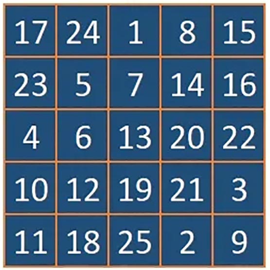
For example, if we create a list of number that increases by 8, as in 8, 16, 24, 32, 40, 48, 56, 64, 72, etc., and then cross-sum them, as follows:
 We get a resulting sequence of 8, 7, 6, 5, 4, 3, 2, 1, 9 which continually repeats itself.
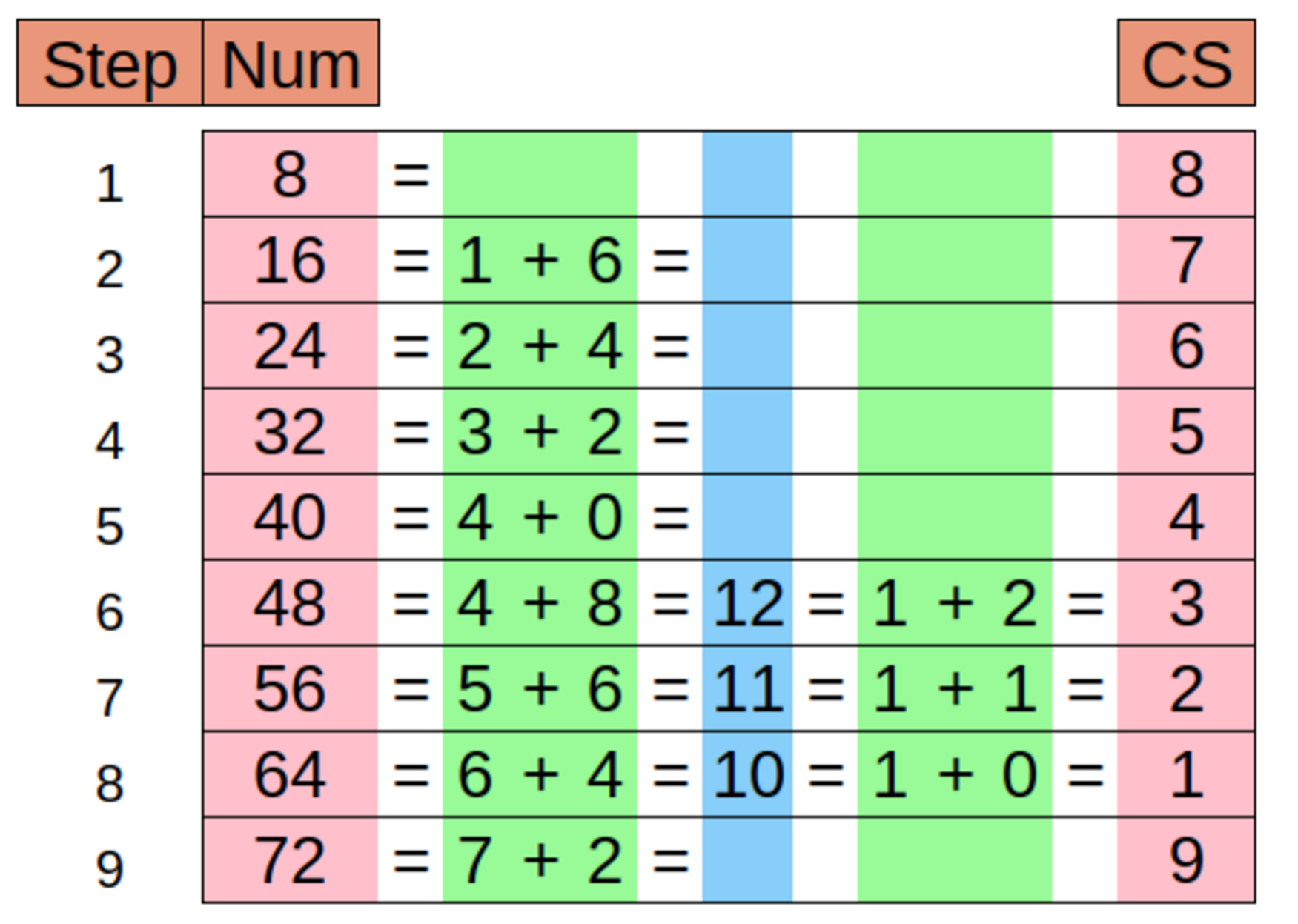
Our original data was sequential because it was tracking the linear movement of planets, so that means that the progression of values will always represent progressive points on a linear path, with each value being slightly larger (in this case) than the previous value, but when we cross-sum these values, all spacial or temporal information is lost leaving only the pattern of the relationship of the numbers. For example, 10 is larger than 9, but cross-sums to 1. Here, 1 represents the lower octave (for lack of a better term) of 10. Cross-summing essentially lowers all the numbers to the same octave. We see this in the number matrix below (left), as any consecutive sequence of digits will always repeat one of the nine patterns shown in the matrix. While this removes a lot of quantitative data, it does not remove the relationship between the data. In fact, it makes that relationship clearer, much like listening to a ten octave piano piece in only one octave.
This number matrix shows the repeating pattern of every sequence of numbers that increases by the number in the left column. The chart on the right shows the changing progression of each of the rows in the matrix is actually only 6 stages of transformation between the straight line at the bottom (1) and the perfectly ordered line at the top (8). The line above that (9) are the totals of each line, which also happens to be exactly the same pattern as line 8. The graph at the bottom shows these same numbers but non-stacked and smoothed, and here you can see the symmetry of the progressive changes. This example applies to any sequence of integers.
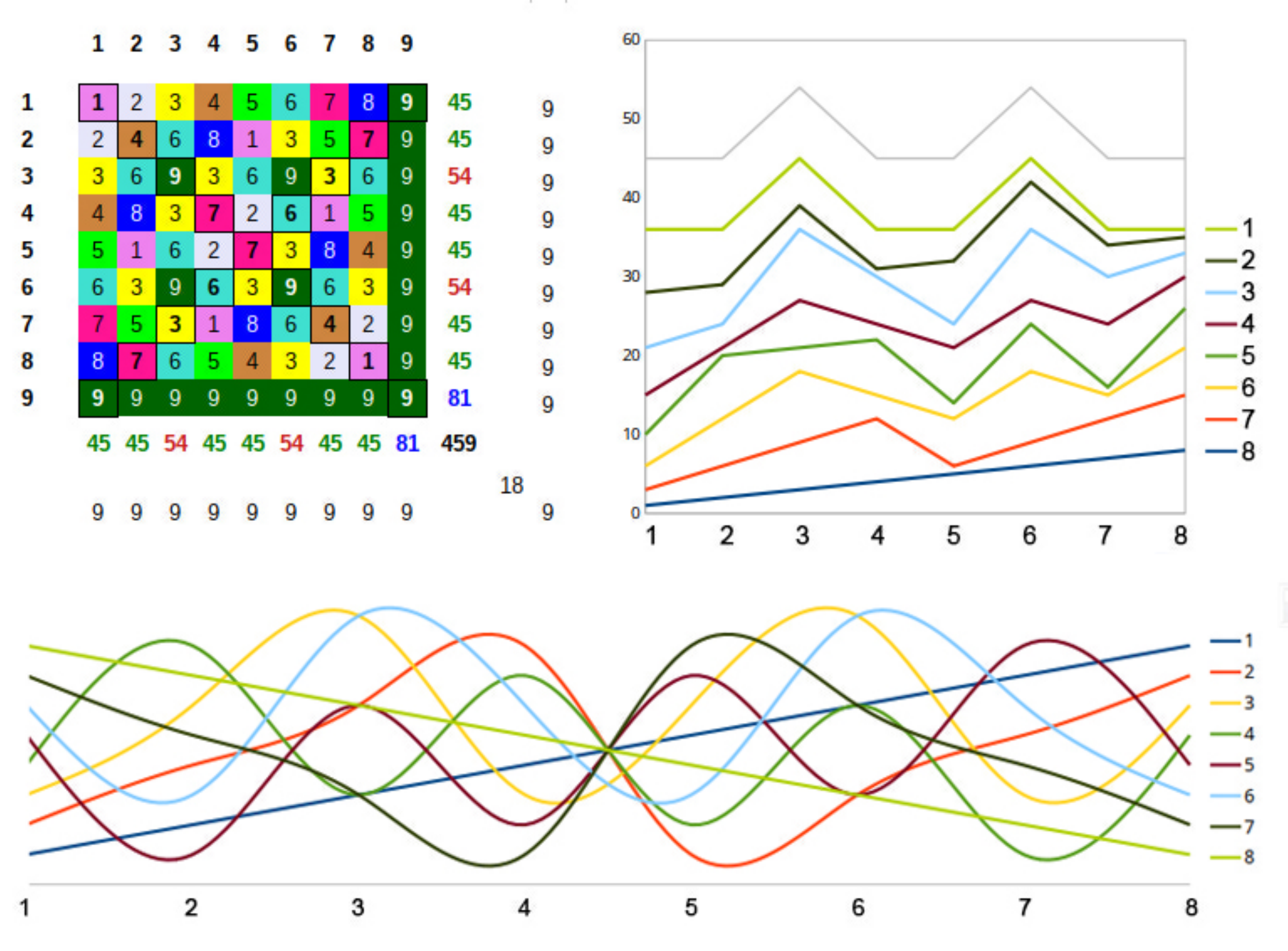
In our example of the series of numbers based on multiples of 8, we have two types of numbers; the quantitative values and the cross-summed values that represent their “position” or relation to other numbers within the context of a base-10 number system. In the charts below, the top-left chart below shows both of these values as two dimensional. and also shows how as the quantitative value increases the cross-sum value can decrease. The top-right chart shows the values of two dimensions plotted as x and y values which shows the that the difference between the diverging values is linear.
Further below, the left chart is a plot of what appears to be un-patterned data, but when we reduce it to one octave by cross-summing, we see a very clear pattern.
The point of this is to demonstrate how there can be hidden patterns in seemingly un-patterned data that has nothing to do with how it exists in time and space.
Attempts were made to replicate the patterns that appeared in the planetary data with various other inputs, such as incremental counting, the number of seconds from some moment, a number and some function of that number, such as square root, but nothing was able to get even close to the Sun/Moon patterns. This suggests that the Fresnel pattern is not solely an inherent pattern of cross-sums, but is a result of the source data. If that is the case, could it be possible that the Fresnel pattern is a property of the movement of the Sun and the Moon or at least two rotating bodies in the same system?
The image below is more fun than informative because it fuels the imagination. These are two top charts that show 64 samples of the position of the Sun to 14 places. The values of each place are then plotted as one set of data. For example, if there are three samples of data of 1.23, 4.56, and 7.89, we plot the 1st line as 1,4,7, the 2nd line as 2,5,8 and the 3rd line as 3,6,9. Were this a live, real-time plot, we would see the outermost circle (or top-most line), changing thousands of time a second, and the innermost (or bottom) changing every couple of months. If we plotted time instead of space to 14 places, the outer (or top) would change a million times a second, and the inner (or bottom) would change once every 11 days. It is very interesting (although probably statistically meaningless) that (in the upper left image) there is an obvious pattern in the first 6 values, and with the 7th, that pattern completely falls apart. Compare the image in the next diagram, Image 3 , “CS patterns to 18 places”.
The bottom 2 images are simply a graph where each value is a dot over the course of 3,000 samples. You’ll notice that the pattern is remarkably identical to the image titled “Distribution of prime numbers for each of the 53,041 ‘microstates’ of the number 300” at the end of the chapter titled “The Thologram”, where we apply the concept of entropy to numbers.
The following images were created by plotting each digit of the position of the Sun.
- In Img. 1, we begin with the first number at the bottom. Each subsequent digit is plotted 3×number degrees to the left or right, with even numbers to the right, odd numbers to the left. For example, the number 9 would be plotted 27 degrees to the left, and the number 8 would be plotted 24 degrees to the right. The width of the line is relative to the digit’s place, so 1.0 is wider than 0.1 which is wider the 0.01, etc. The image below, Img. 1a, is the same algorithm but based on random numbers rather than the Sun’s position, and each new position of the Sun moves down the X-axis. The purpose of this graph is to visually show the expanding scope that starts from one point. The reason for odd=left and even=right was to see what pattern we would get if we used the traditional yin/yang and ancient Greek concept that even numbers are yin in nature and odd numbers yang in nature1. If there was any validity to this then we would expect to see a pattern common in nature, which is exactly what we get. Img. 1b is the same as Img. 1a, but where the initial direction of each like the plot is random.
- Img. 2 is similar to Img. 1, except each number is plotted adjacent to the previous number (and the colors were changed, the deviation was lessened, and the length of the plot was slightly shortened).
- Img. 3 is something quite different. Rather than using the position of the Sun, we used the recurring cross-summed patterns of the sequence of numbers when we increase counting by 1 through 9 (as shown in the number matrix above). The image below, Img. 3a, is that same sequence but with a much larger value so as to see its larger pattern. Interestingly, we end up with three distinct groups; 2,5,8 (cross-sum=6), 1,4,7 (cross-sum=3), and 3,6 (cross-sum=9). The number 9 is all alone by itself and is at the center.
Nishiyama, Yutaka. “A Study of Odd- and Even-Number Cultures.” Bulletin of Science, Technology & Society 26, no. 6 (2006): 479-84. doi:10.1177/0270467606295408. ↩