An Unexpected Pattern
Why does the path of the sun create patterns that describe the refraction of light and the grain of wood?
It’s more them remarkable that patterns in trees follow the same rules as the diffraction of light, and that both of these patterns can be determined by the Moon’s relationship to the Sun… it’s living proof of the idea that every that exists is the same expression of energy within different contexts.
(Most of this is from Appendix F - An Unexpected Pattern in the book THOLONIA)
An Unexpected Pattern
What is this pattern and why does it exist?
In the course of writing this book there was the need to generate sets of chaotic numbers from other sets of patterned numbers. In one case, the results presented a very unexpected pattern.
Numbers were generated by periodically calculating the longitudinal position of the Sun and the Moon (from Earth’s coordinates of -34.61262S, -58.41048W, Buenos Aires, Argentina on the 24th of each month at 5:31:07 PM UT) down to 10-15 radians. The individual digits of these two values were then concatenated, or cross-summed. For example, the Sun’s longitude in radians at one moment was 4.2430033683776855, and the Moon’s position at that same moment was 2.399298667907715. These were then cross-summed until they are reduced to a single digit value.
- 4+2+4+3+0+0+3+3+6+8+3+7+7+6+8+5+5=74
- 2+3+9+9+2+9+8+6+6+7+9+0+7+7+1+5=90
- 74+90=164
- 1+6+4=11
- 1+1=2
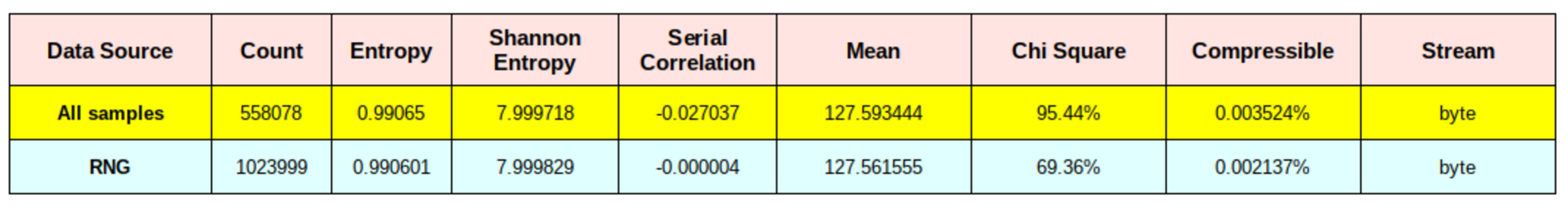
Millions of samples were recorded and reduced to one number per sample. The input data of the Sun and Moon positions was perfectly non-random and linear, but the single cross-summed number series of data was “mostly random” according to the Chi squared results of a randomness test1. Below are the test results of the single-number data and the data from a random number generator (RNG), for comparison2,3.
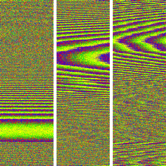
Next, each single digit number (1-9) was assigned a color from the spectrum and then plotted such that each dot occupied one consecutive pixel on one line, and when that line was full, the plot advanced to the next line, just like a dot-matrix printer. This was an extremely simple plot. The below-left plot shows only one number being plotted at a time, and the below-right plot shows cumulative numbers. The distribution of the numbers within the data set of 33,000,000 is shown in the bar chart.
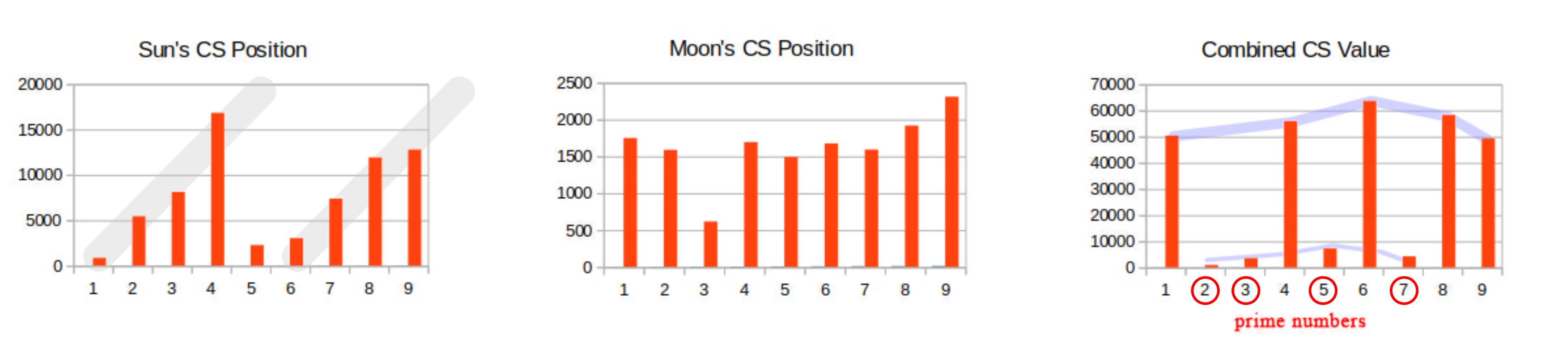
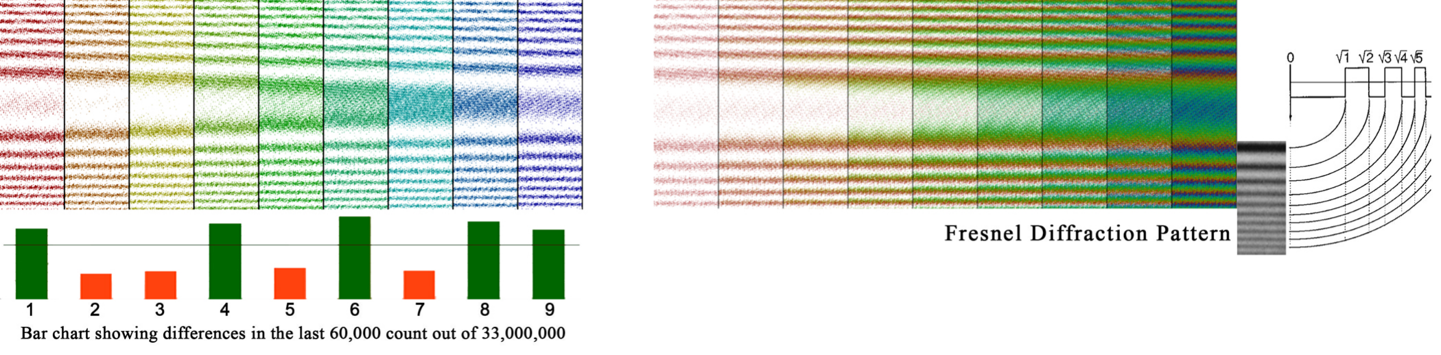
The data was also tested against Benford’s Law, which states that the first digit in a naturally occurring set of values will be distributed in a manner dependent on the log of that number. I tested three sets of data; the crossed-sums of the Sun, Moon, and combined, by counting the number of each digit 1 through 9 in a data set of 33,575,635 data samples. While the numbers were similar in count, they were not similar enough to suggest an even distribution as we would see in random numbers, and not in accordance with Benford’s Law. To see the difference in these totals, I plotted the difference between the lowest and and highest counts (charts below) for each number 1-9. As you can see, there is some very patterned behavior, especially in the first chart and even more so in the last chart which show a very interesting pattern among prime numbers .
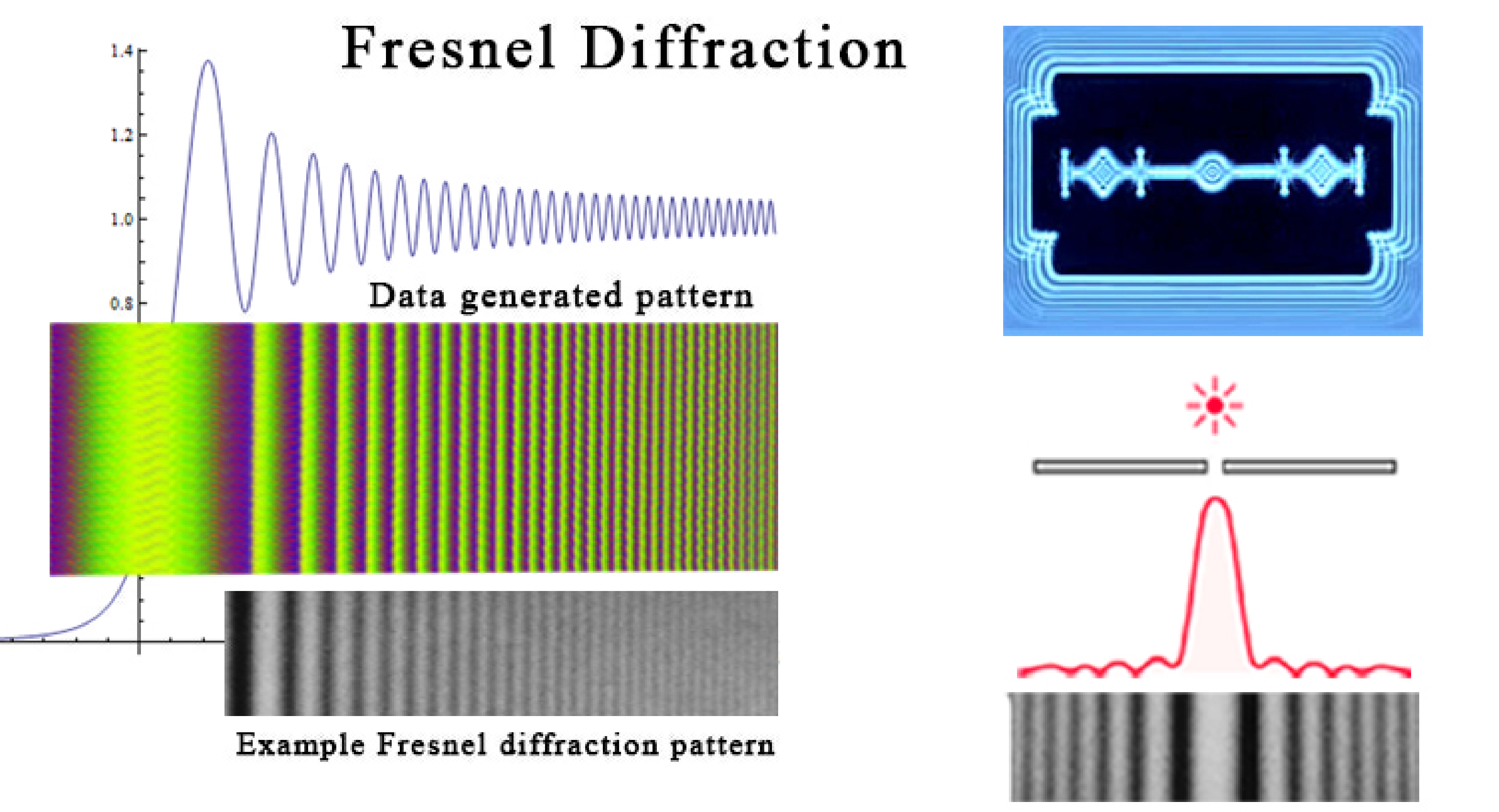
Much to our surprise, this resulting pattern matches that of a Fresnel diffraction.
At the rate of sampling used, each position of each “planet” was only about 7x10⁻⁸ radians further than the previous position sampled. This equates to about 23 kilometers of movement for the Sun and only 64 millimeters of movement of the Moon.
When cross-summing numbers, the place of each digit is insignificant, so 123 and 321 are the same as they both cross-sum to 6. Because all the digits in a cross-summed value have equal significance, the slightest measurable movement of the sun is equal to the movement of the two-thousand years it takes to pass through a constellation. This is because 0.000000000000001 is the same as 100000000000000.0
Above are plotted the values simply as colors, but when the actual values of the cross-summed numbers are used as the Y-axis, with each number advancing one step across the X-axis (time), we get a different perspective, as seen in the top image below. The bottom image is the same plot but only using the differences between each number.
This plot uses 300,000 cross-summed data points that covers 25 minutes of observation.
What was surprising is that the top image appears to be a the cross-sectional diagram of a Fresnel lens!
This raises the questions:
- Where do these patterns come from?
- Do they tell us anything about the thing being measured?
- Given that these patterns are the same that describe the propagation and near-field diffraction of light (i.e. Fresnel diffraction), can we apply any other attributes of light to whatever we are observing?
Additional details for the curious
Below are some of the visual results of the plot.
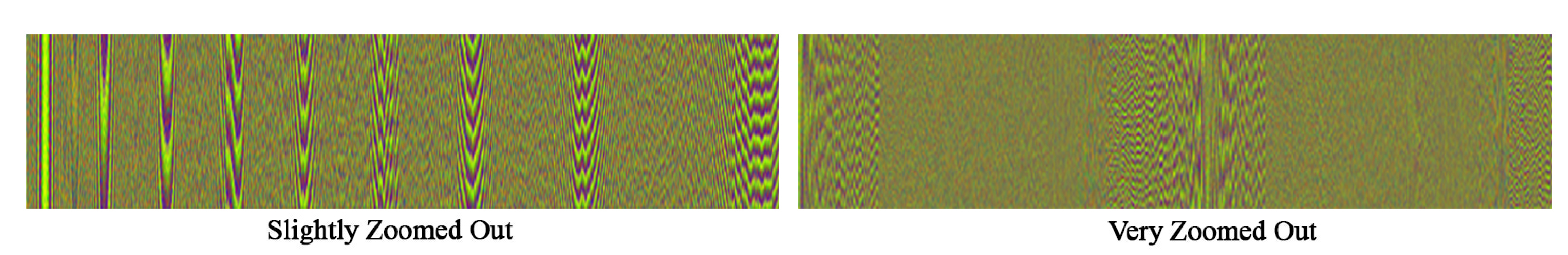
These plots are of data captured every 0.005 and .01 seconds and we only are looking at the cross-summed values that are prime numbers (2,3,5,7), but the results were the same when using all number 0-9. These twelve plots represent sampled data from each month of the year at the same time.
 It is interesting to see how the 0.005s look slightly “zoomed out” compared to the 0.01s. Also interesting is how the plot pattern and the pattern of wood grain is so similar, suggesting the source of these patterns also share a common process. at least mathematically.
If we change the time between samples from microseconds to days, we see another pattern. Below are ten sets representing ten months with the same starting point as the sets above, but each pixel represents an entire day (86480 seconds), i.e., the position of the Sun and the Moon was recorded only once a day. This means that the entire set represents 1,095 years. Each plot looked almost identical and appeared completely random, but upon closer examination, they were not random at all, but a very “zoomed out” view. It is clearer to see the pattern if we only show the blue dots of a small section of the image.
My first assumption was the farther “out” we zoom, in time, the clearer the patterns, but it seems to be the exact opposite; the smaller the time delta, the larger the pattern. This might make sense if we were looking at the linear difference between, say, 1.234567 and 1.2345678, as the difference would be 0.0000008, and such a small change would need a lot of samples to make itself apparent, but this does not apply here because we are cross-summing the numbers together, making the place of the digits meaningless.
Below is a comparison of the patterns at each scale. The values above the images are the interval sampling time, and the values below is the entire duration of the sample. No obvious pattern can be seen at 5s, but a slight pattern begins to emerge at 0.5s, becomes more clear at 0.05s, and is most dominant at 0.005s. A pattern is equally visible in 0.0005s, but it appears only as a simple oscillation or wave. 0.00005 is identical to 0.0005 because (it seems that) once we start going below 0.002, we hit the limits of resolution. This is the point where we begin getting duplicate data because the Sun or Moon has not moved enough in the small amount of time between samples, and the smaller we go the more duplicates we get. For example, at 0.00001 second intervals of sampling , to get the 155,520 unique data points to create the graph, we need to sample 50,000,000 times. This simple wave pattern is the first wave pattern we can detect (given the limitation of my laptop and/or the ephemeris used to calculate planetary positions). This simple wave pattern is what then evolves into the more complex patterns. Presumably, the difference between sample points in the wave patterns is only the rightmost last digit being increased by 1, given that we keep sampling until we get the next unique number.
How do we have patterns when we sample of 0.01, but nothing (significant) when we sample as .05? I think this has to do with where we are sampling from within the entire pattern. The two images below shows that the Fresnel pattern is slightly altered with time, but eventually returns. At its most ordered point it looks like Fresnel diffraction, but at its least ordered point it looks identical to pure random data (but we assume it is just as ordered, only difficult to see that order).
When the data is sampled we have no idea where within the cycle of repeating patterns we are, so it is only by chance that we will end up in an ordered section.
For those not familiar with Fresnel diffraction, it is the way that light interferes with itself as it travels around the edge of an object
Digging Deeper
Having no idea where to look for more information, I posted this to various mathematics forums, and even though the question was read by many, no one had an answer. I then sent this question to my old friend who is an accomplished physicist, but who also considers these speculative ideas to be a waste of time, so I knew any answer he gave would include an unabashed commentary on the silliness of it all.
He did not disappoint on either front. I’ll forego the commentary and just focus on the relevant part of his reply, which was very short. Essentially he told me that no matter how hard you try to create random numbers from non-random data, you will always end up with some sort of a pattern. “Why?” was my naive response, to which he replied only “Look into Zipf’s Law”.
Zipf’s Law is (from Wikipedia):
an empirical law… that refers to the fact that many types of data …can be approximated with [certain types of] power law probability distributions. Zipf distribution is related to the zeta distribution, but is not identical.
There are two very significant points in this definition. The first is that it is an empirical law. Something is called an empirical law when it can be observed, but not proven (yet). The second important detail is that Zipf distribution is related to Zeta distribution. We’ll get to that in a moment.
Zipf’s Law was not discovered by physicists or even within the hard sciences. It was a French stenographer, Jean-Baptiste Estoup (1868 - 1950) that first discovered the patterns of words which became Zipf’s Law after it was popularized by the American linguist George Kingsley Zipf (1902 - 1950).
It seems that languages, all languages, from every corner of the world, both modern and ancient, follow Zipf’s law in the way words are distributed in both writing and speaking (and by inference, some implicit pattern in the way we think). We don’t need to drill into the details, but what is significant is that this same distribution pattern is also seen in city populations, solar flare intensities, protein sequences and immune receptors, the amount of traffic websites get, earthquake magnitudes, the number of times academic papers are cited, last names, the firing patterns of neural networks, ingredients used in cookbooks, the number of phone calls people received, the diameter of Moon craters, the number of people that die in wars, the popularity of opening chess moves, even the rate at which we forget… and countless more.4
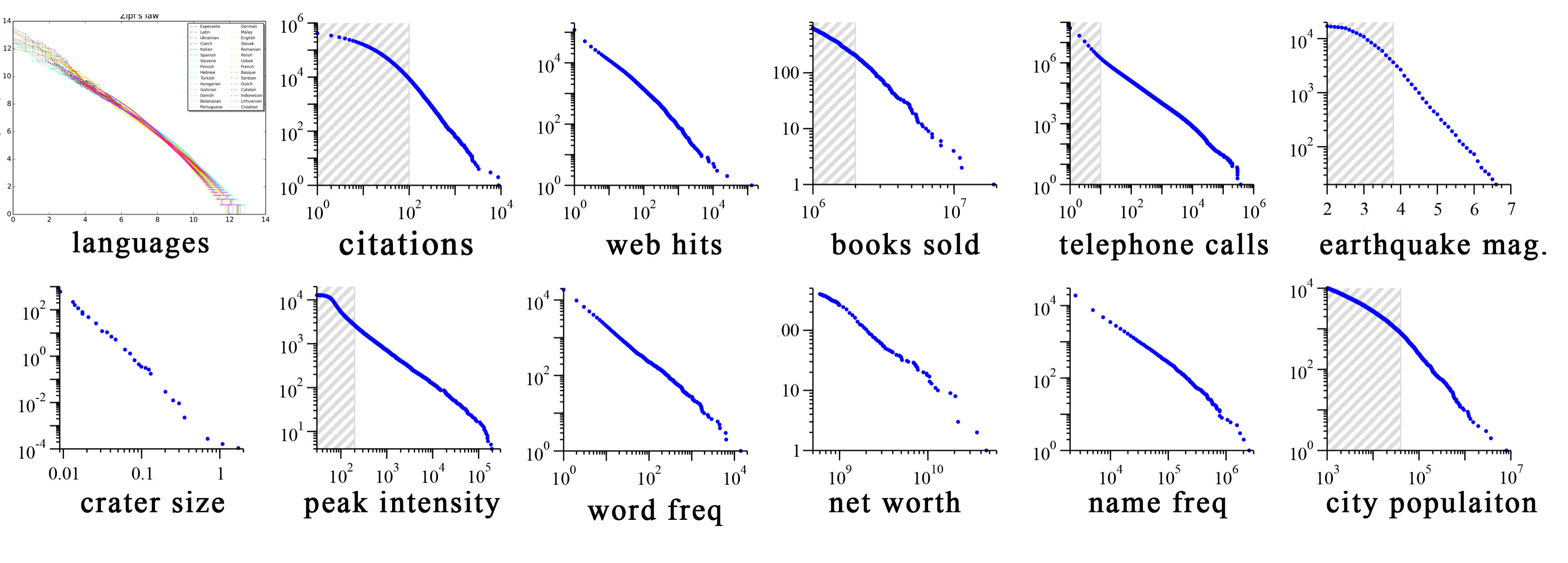
In short, Zipf’s law is an example of power laws, and power laws touch everything in existence in one way or another. But what does this have to to with anything? This is where the second point applies. The charts above are called Zipf Distributions, and they all have different scales of values based on the kind of data being sampled. If we reduce all the scales to 1, we have what is called a normalized Zipf distribution, also known as a Zeta distribution. Mathematicians use the Riemann zeta function (RZF) to study and test these distributions. This function is written as ζ(*s*), where s is any complex number other than 1.
 Related sidenote, using just prime numbers you can also determine π, but this has nothing to do with RZF:
  .
.
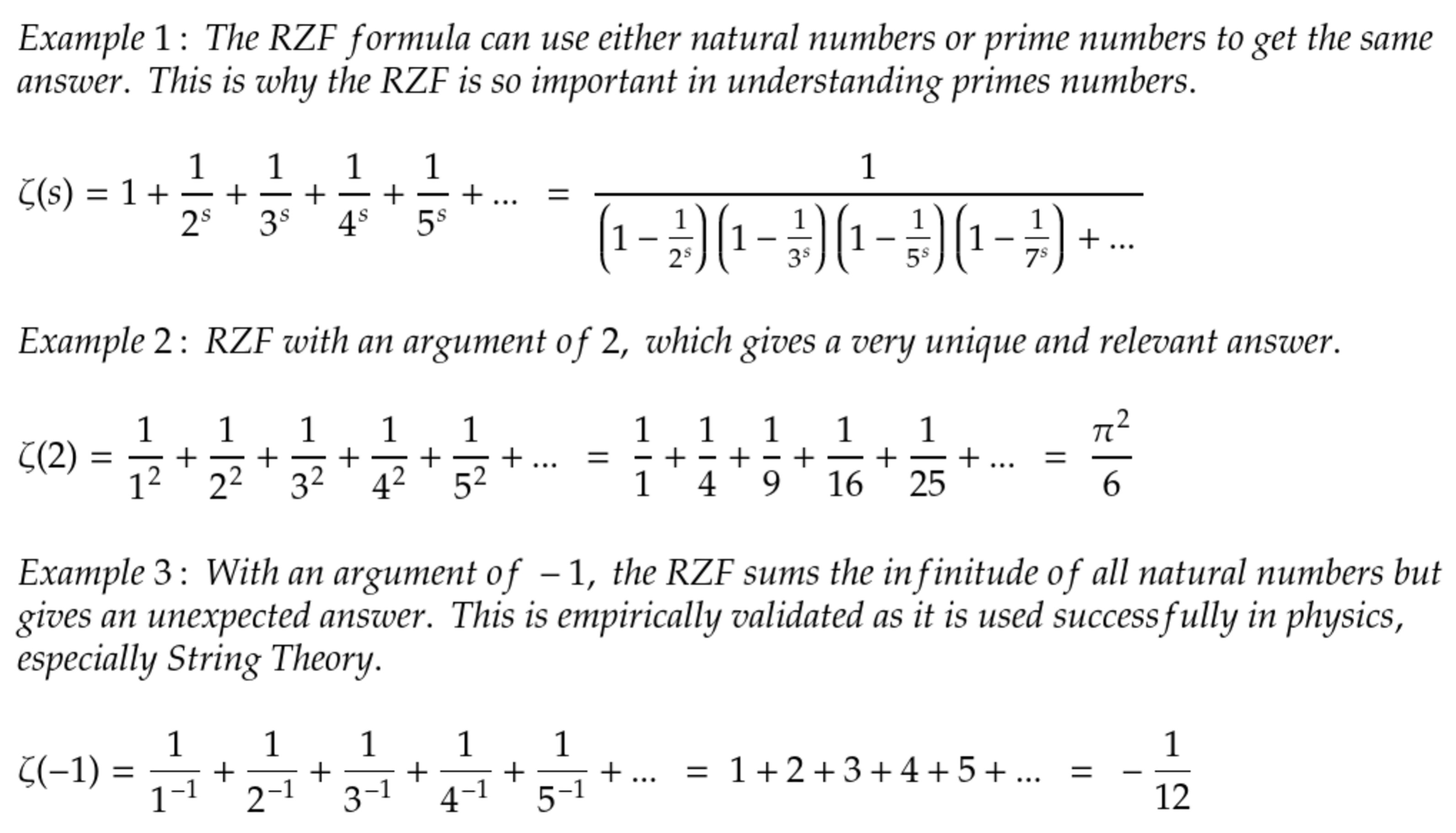
One of the useful features of the RZF is that it can turn a divergent series of numbers (numbers that when you add then together approach infinity) into a convergent series (when the sum approaches a specific value, like  or
or  ). It can do this because the hypothesis uses the concept of analytic continuation and complex numbers. You can play with this function using an online Riemann Zeta Function Calculator. 5
The RZF is based on the Riemann hypothesis, which also states that ζ(s)=0 only when s is a negative even integer or a complex number with real part of  . This hypothesis is really quite profound in the way it relates to the distribution of prime numbers. That won’t be explained here, but it is understandable when properly explained. There are a couple of excellent videos on the subject here and here.
This 160-year-old hypothesis has yet to be proven, however, and because it is considered by many mathematicians to be the most important unsolved problem in pure mathematics, the Clay Mathematics Institute has a reward of US $1,000,000 to anyone who could solve it. (Update. September 24, 2018. Michael Atiyah , the 89 year old mathematician emeritus at The University of Edinburgh, claims he has proved this, but many experts doubt its validity)
Understanding how the RZF works would (probably) help explain the how and why patterns of numbers appear organically in any data-set of naturally occurring samples, such as the charts above.
What value would we get if we applied the RZF to the series of square roots of natural numbers, the same numbers that define a Fresnel diffraction? Some really smart person did exactly this 6, and the answer is… voilà!

This is the inverse of  , and is especially interesting because now we have a formula that fits into Ohm’s Law and Newton’s laws of motions.
(content omitted as it is only relevant for other topics in the book)
The Cornu Spiral
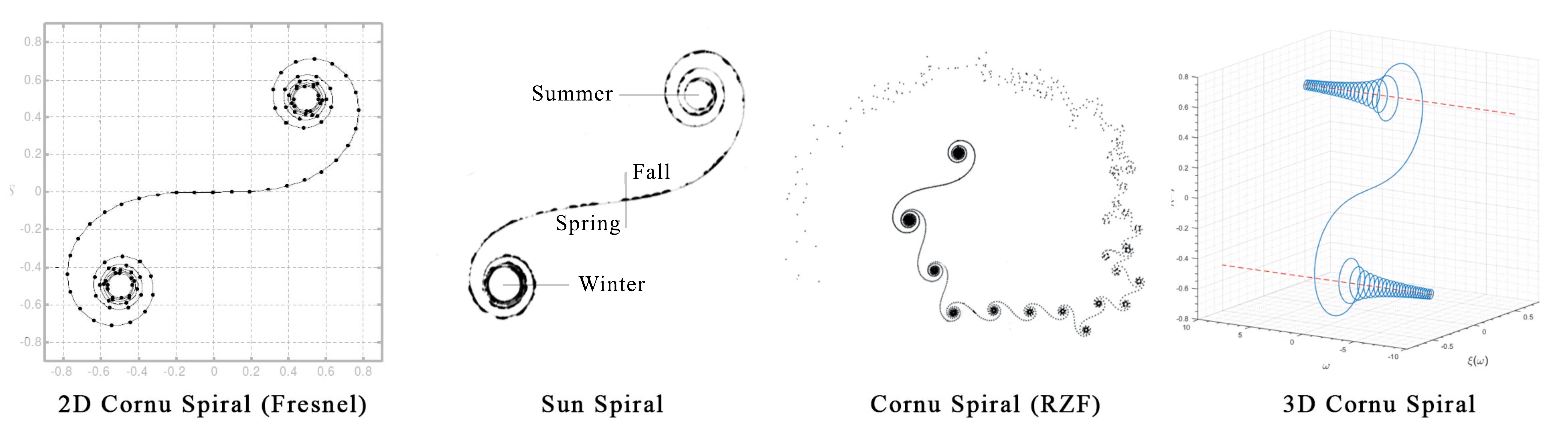
While the manner in which the cross-summed numbers create a diffraction pattern may be a mystery (to me), how diffraction patterns are created are not. Properly described, it would require a lot of math which we won’t get in to here, but a quick search on “What is the Cornu’s spiral method for diffraction pattern?” will reveal all to the more curious. In short, because we know that the intensity of light at any point is always proportional to two values known as the Fresnel integrals 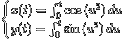 , we can plot the intensity of each point along the diffraction pattern on a 2-Dimensional plot. When we do this, we end up with an amazing figure called the Cornu Spiral, shown below as “2D Cornu Spiral (Fresnel)”.
Another interesting thing about the Cornu Spiral is that it also describes the path of the sun over the course of the year (from Earth’s perspective)7, which is pretty poetic. It appears as though the Cornu spiral describes not only how light and matter interact in the nanometer scale, but also on the planetary scale, at least in one sense.
Not surprisingly, the Riemann Zeta Function also creates not just one Cornu Spiral, but an entire series of spirals, as shown in “Cornu Spiral (RZF)”, that emerge from nothing and continues to expand from within itself.
The x and the y values are the result of a function based on a single value, as in x(t) and y(t) of the Fresnel Integrals, but there can be a third dimension based on t. When this new z(t) dimension is proportional to the x and y dimensions, a cone is created on the z-axis, which might be related to the diminishing angles of the diffraction pattern in the “Slightly zoomed out” plot of the cross-summed data patterns shown above.
So, by saying the following…
- The Cornu Spiral describes the diffraction pattern.
- The RZF describes a Cornu spiral.
- The RZF is a normalized version of the the Zipf Function.
- The light of the sun hitting Earth creates a Cornu-ish spiral over the course of a year.
… we can relate our mystery pattern to quite a few other patterns, including Newton’s 2nd, but the most dominant have to do with the nature of light.
In one way, it is like the cross-summed numbers are similar to photons in that it is the individual photons that create the diffraction pattern just like the individual numbers of our data also create the diffraction pattern. Both of these “particles” (photons and numbers) are presumably following some of the same rules in some fashion if we are to judge them by their resulting patterns. Given my lack of training in this area, I can only wonder if the wave/particle properties of photons also apply (contextually) to cross-summed numbers, or numbers in general. Perhaps they are somehow related or similar to Feynman Sunshine Numbers, which relates prime numbers and photons, among other things? These are numbers that include RZF values that appear in the description of sunshine as well as ancient relics of the Big Bang, and the theory of photons, electrons and positrons.
##
Footnotes
These tests are: monobit frequency test, block frequency test, runs test, longest run ones10000, binary matrix rank test, spectral test, non-overlapping template matching test, overlapping template matching test, Maurers universal statistic test, linear complexity test, serial test, approximate entropy test, cumulative sums test, random excursions test, random excursions variant test, cumulative sums test reverse. These tests are provided by the National Institute of Standards and Technology as implemented by the program testrandom.py by Ilja Gerhardt, https://gerhardt.ch/random.php. The numbers published here are the result of the program “ent”, a a pseudo-random number sequence test program by John Walker of Fourmilab Switzerland, https://en.wikipedia.org/wiki/John_Walker_(programmer) ) ↩
Data generated with the command “ent” with the following variables: Is Intel CPU; AESNI Supported in instruction set; Format=Hex model=pure size = 1000 kilobytes XOR mode off XOR range mode; off Output to file x Hardware Random Seeding on. Non deterministic mode; Reseed c_max=511; Using RdRand as nondeterministic source; Total Entropy = 0.000000; Per bit Entropy = 0.000000 % ↩
These tests are: monobit frequency test, block frequency test, runs test, longest run ones10000, binary matrix rank test, spectral test, non-overlapping template matching test, overlapping template matching test, Maurers universal statistic test, linear complexity test, serial test, approximate entropy test, cumulative sums test, random excursions test, random excursions variant test, cumulative sums test reverse. These tests are provided by the National Institute of Standards and Technology as implemented by the program testrandom.py by Ilja Gerhardt, https://gerhardt.ch/random.php. The numbers published here are the result of the program “ent”, a a pseudo-random number sequence test program by John Walker of Fourmilab Switzerland, https://en.wikipedia.org/wiki/John_Walker_(programmer). ↩
Stevens, M. (2015, September 15). The Zipf Mystery. Retrieved June 30, 2020, from https://www.youtube.com/watch?v=fCn8zs912OE. The page of this video has dozens of excellent related links ) ↩
https://solvemymath.com/online_math_calculator/number_theory/riemann_function/index.php or https://keisan.casio.com/exec/system/1180573439, for example ↩
Snehal Shekatkar, The sum of the r’th roots of first n natural numbers and new formula for factorial, 2012, arXiv:1204.0877v2 [math.NT], [https://arxiv.org/abs/1204.0877v2()]https://arxiv.org/abs/1204.0877v2) ↩
Saad-Cook, J., Ross, C., Holt, N., & Turrell, J. (1988). Touching the Sky: Artworks using Natural Phenomena, Earth, Sky and Connections to Astronomy. Leonardo 21(2), 123-134. https://www.muse.jhu.edu/article/600628. Charles Ross, the creator, describes: “1972. I had placed this simple lens set-up on the roof so the sun would burn a path across a wooden plank as the day progressed. The idea was to collect a portrait of the weather each day. As the work progressed, I noticed that the burn’s curvature was changing with the seasons. We took photos of the burns and placed them end to end following their curvature to see what a year’s worth looked like. The sum of days generated a double spiral figure. At first, it did not make any sense-this primitive lens set-up was producing a complex spiral shape. A few of the astronomers I showed it to said, “Well, it must be coming from somewhere, but we have no idea what it is”. Most of the scientists insisted that there had to be some anomaly in the set-up and that the shape had nothing to do with astronomy -just some weirdness in the lens. In reality, it made no difference at all if the lens faced one way or the other as long as it faced generally toward south. The elements of the spiral are in sunlight itself; it was an archetypal image falling from the sky. I finally contacted Kenneth Franklin at the Hayden Planetarium. He directed me to the Naval Observatory, where LeRoy Doggett, an astronomer with the Nautical Almanac office…”. Authors note: This Sun Spiral was pieces together manually from many separate samples, and should not be seen as an accurate representation of the suns paths, but only an approximation. ↩